The Asset Administration Shell (AAS) is an emerging concept in connection with the digital twin data management. It is a virtual representation of a physical or logical unit, such as a machine or a product. The AAS enables relevant information about this unit to be collected, processed and used to ensure efficient and intelligent production. The architectural standardization of the AAS enables communication between digital systems and is therefore the basis for Cyber Physical Systems (CPS). You can find out more about the need for digital twins in the industry here: ZEISS Digital Innovation Blog – The digital twin as a pillar of Industry 4.0
The following article focuses on the actual implementation of an example. In one scenario, we will use a reference implementation from the Fraunhofer Institute for Experimental Software Engineering IESE (BaSyx implementation of AAS v3) to establish an information exchange between two participating partners. For the sake of simplicity, both parties are based within one company and share the infrastructure.
Note: This application is also suitable for cross-company distribution. The respective security aspects are not part of this scenario.
Scenario
Factory A is a manufacturer of measuring head accessories and produces pushbuttons, among other products.
Factory B manufactures measuring heads and would like to install pushbuttons from factory A on its measuring head.
In addition to the physical forwarding of the pushbutton, information must also be exchanged. The sales department of factory A provides contact information so that the technical purchasing department of factory B can access and negotiate prices. Moreover, factory A must also provide documentation, etc.
For this exchange of information:
Contact details and
documentation
the AAS concept is to be used.
Infrastructure
In our scenario, we want to use type 2 of the Asset Administration Shell. Here, the AAS is provided on servers and there is no exchange of AASX files, but rather communication between the different services via REST interfaces.
In our scenario, the different services run within a Kubernetes cluster in Docker containers.
AAS repository, submodel repository and ConceptDescription repository are provided within one container – the AAS environment.
Technical implementation
The communication is only done via API calls to the corresponding REST interfaces of the services.
For this, we will use simple Python scripts to represent a communication in which the manufacturing factory B wants to receive information about a product (here: a pushbutton for a sensor) from the component factory A.
Procedure
Factory B only knows the asset ID of one pushbutton, but knows nothing else about this component.
Factory B uses the Asset ID to request the discovery service in order to obtain an AAS ID.
This AAS ID is used for requesting the central AAS registry, which provides the AAS repository endpoint of factory A.
Via this endpoint and the AAS ID, factory B receives the complete Asset Administration Shell including the relevant submodel IDs.
With these submodel IDs (e.g., for contact details and documentation), factory B requests the submodel registry of A and receives the submodel repository endpoints.
Factory B requests the submodel endpoints and receives the complete submodel data. This data includes the desired contact information for the buyer and complete documentation for the pushbutton asset.
The process is illustrated in detail below using UML sequence diagrams.
UML sequence: Creation of AAS registration in component factory A
Factory A is responsible for registering its own component.
Figure 1: UML sequence: Creation of the AAS registration in component factory A
UML sequence: Requesting the component data
Factory B requires data about the component and requests it from the AAS infrastructure. Here, factory B may only have access to the asset ID of the component, in our case that of the pushbutton.
Figure 2: UML sequence: Requesting the component data
Implementation
For the process described above to work, the services mentioned must be made available. Secondly, shells and submodels must be created and also stored in the registries.
Service deployment
Deployment takes place via Docker containers that run within a Kubernetes cluster. For this, each BaSyx image receives a Kubernetes deployment which starts the corresponding pods via Kubernetes replica sets. By means of port forwarding, for example, the corresponding ports are made accessible by the host. This is necessary to address the APIs according to the example Python scripts.
A relatively simple Kubernetes deployment configuration looks like this. There are four deployments, each with a replica set.
Figure 3: Kubernetes deployment configuration
Creating the AAS from factory A
Factory A would like to provide the contact details for its pushbutton component, for example.
For this, submodels are created in the AAS repository (here: in the AAS environment) and registered in the submodel registry.
Subsequently, the Asset Administration Shell is created in the AAS repository and registered in the AAS registry.
The shell reference is then added to the AAS repository.
This completes the registration process from the component factory.
Contact details requests from factory B
Factory B would like to receive the contact details and requests the various AAS services according to the workflow described above. Ultimately, the submodel data set containing the required values is obtained and can then be made available within a user interface, for example.
Conclusion
The Type 2 Asset Administration Shell is a distributed system that is based on the corresponding repositories, registries and the discovery service. In our example, we have only used a simple submodel template for contact data. However, there are far more templates available for many applications.
Communication between the services for the provision and retrieval of data is relatively straightforward, although aspects such as security were not a focus in this scenario.
The example implementation described in this article gives an idea of the immense potential of the AAS concept and encourages users to start concrete implementations.
This post was written by:
Daniel Bruegge
Daniel Brügge works as a software developer at ZEISS Digital Innovation with a focus on cloud development and distributed applications.
Computers and automation technology began to gain a foothold in the production industry in the 1970s, making it possible to set up flexible mass production options in locations away from physical assembly lines. With the advent of this technology, machines were optimised to ensure maximum workpiece throughput. This process, which continued into the 2000s, is generally known as the third industrial revolution.
Industry 4.0 – as it was coined by the German government and others in the 2010s – has different aims, however. Since machine uptimes and entire production lines in many industries are already being optimised as much as they possibly can, attention is now turning to the methods that can be used to optimise downtimes – a term that is primarily used to refer to points in production when machines are at a standstill or are producing reject parts.
Two major approaches to optimising downtimes
100% capacity utilisation as a goal for every machine
If my production machines aren’t doing what they were purchased and installed for, they are not being productive and are not adding any value. There are two types of downtime to consider: planned and unplanned. To ensure that no time is wasted even when downtimes are taking place as planned, machines can be deployed flexibly at several points in the production chain – resulting in more of their capacity being used overall. A good example of this is a six-axis robot with a gripper that can be moved from one workstation to another as needed, working on the basis of where it can be put to good use at that point in time. This approach uses the concept of changeable production. Unplanned downtimes, meanwhile, usually happen as a result of component or assembly failures within a machine. In these cases, machine maintenance needs to be scheduled so that it is only performed at the times when planned maintenance is due to take place anyway (as part of predictive maintenance measures).
Reducing rejects
Another major approach involves reducing the amount of rejects produced: this also makes it easier to perform the process monitoring stages that take place after a production cycle (or perhaps even during it). Process control builds on the process monitoring stage, feeding the findings it gains back into the production cycle (process) in order to improve the outcomes of the next cycle. It is easy to visualise how this could take place in a single milling cycle, for example: after a circle outline has been milled, the diameter of the circle is measured and then evaluated. If there are any deviations, the milling programme can then be adapted for the next part undergoing the process. More complex approaches aim to manage process monitoring across multiple steps – or perhaps even multiple steps distributed across multiple subcontractors.
Data: the key to more efficient planning
Improved planning and control over processes are important elements in both of these approaches to optimising production. To improve planning, it is vital to have a significantly increased pool of data that is highly varied and needs to be analysed in specific ways, but the sheer volume and level of detail involved in this kind of data far exceed the capacity of humans to perform the analyses. Instead, complex software solutions are needed to derive added value from data.
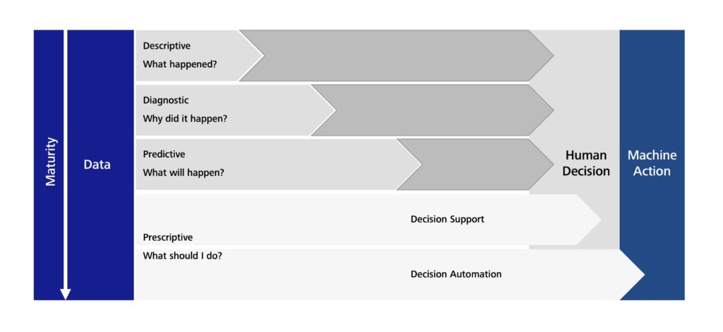
Depending on the level of maturity of both the data and the analyses, software can be a useful tool – and is increasingly being called upon – in supporting the work of humans in production environments. The level of input that software has can range all the way up to fully autonomous production. The data analytics maturity model shown in Figure 1 can help you map out what is happening in your own production scenario. It provides an overview of the relationship between data maturity and the potential impact of software on the development process.
Figure 1: Data analytics maturity model. Reproduced with permission from[1]
At the lowest level of the model (Descriptive), the data only provides information about events on a machine or production line that have happened in the past. A lot of human interaction, diagnostics and – ultimately – human decisions are required to initiate the necessary machine actions and put them into practice. The more mature the data (at the Diagnostic and Predictive levels), the less human interaction is needed. At the highest level (Prescriptive), which is what useful systems aim to achieve, it is possible for software to plan and execute every production process fully autonomously.
Aspects of data in digital twins
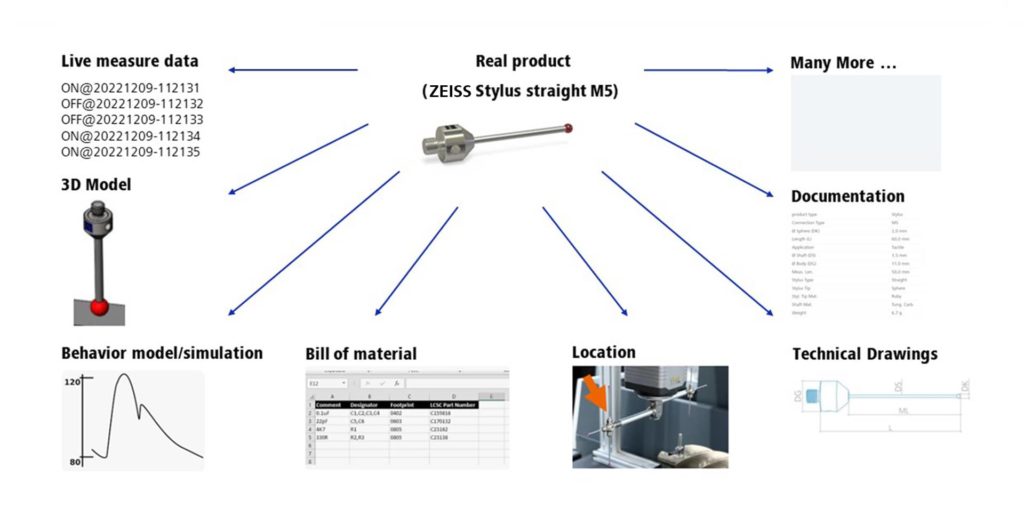
As soon as data of any kind starts to be collected, questions concerning how it needs to be sorted and organised quickly come about. Let’s take the example of a simple element or component as shown in Figure 2. Live data is produced cyclically while this component is being operated within a production machine; however, data of other kinds – such as the bill of materials and technical drawings – may be more pertinent during other stages in the component’s life (during its manufacture, for example). If the component is not actually present but you still want to collect data about it, you can draw on a 3D model and a functioning behaviour model that can be used to simulate statuses and functions.
Figure 2: Various aspects of data shown using the example of the Zeiss Stylus straight M5.
On encountering the term “digital twin”, most people’s minds simply jump straight to a 3D model that has been augmented with behaviour data and can be used for simulation purposes. However, this is only one side of the story in an Industry 4.0 context.
A digital twin is a digital representation of a product* that is sufficient for fulfilling the requirements of a range of application cases.
Under this definition, a digital twin is even considered to exist in the specific scenario I outlined above – which indicates that there are lots of different ways of defining what a digital twin is, depending on your perspective and application. The most important thing is that you and the party you are working with agree on what constitutes a digital twin.
Digital twin: type and instance
To gain a better understanding of the digital twin concept, we need to look at two different states in which it can exist: type and instance.
A digital twin type describes all the generic properties of all product instances. The best comparison in a software development context is a class. Digital twin types are mostly used in the life cycle stages that take place before a product is manufactured – that is, during the engineering phase. Digital twin types are often linked to test environments in which efforts are made to optimise the properties of the digital twin, so that an improved version of the actual product can then be manufactured later on.
A digital twin instance describes the digital twin of exactly one specific product, and is linked explicitly with that product. There is only one of this digital twin instance anywhere in the world. However, it is also completely possible for this instance of a digital twin to represent just one specific aspect of the actual product – which means that multiple digital twins, all representing different aspects, can exist alongside each other. The closest comparison for this in a software development context is an object. Digital twin instances are usually encountered in the context of operating actual products. In many cases, digital twin instances are derived from types (in a similar way to objects being derived from classes in software development).
Digital twins in the manufacturing process
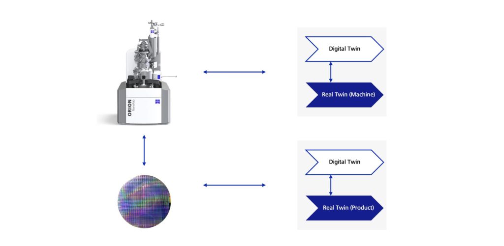
In the context of Industry 4.0 and, therefore, the manufacturing process, it is important to be constantly aware of whether a digital twin is referring to the production machine or the workpiece (product) to avoid any misunderstandings. Both can have a digital twin, but the applications in which each is involved are very different.
Figure 3: Digital twin of a machine and a workpiece. Both scenarios are possible.
If the process of planning the actual production work were the most important aspect of the scenarios I am presenting here, I would be more likely to deal with digital twins of my production machines. If my focus were on augmenting data for my workpiece, and therefore for my product, I would be more likely to turn to a digital twin for the product. There is no clear distinction in how these aspects are used: both approaches can be used for me and my production work, but may also be beneficial for the users of my products.
Categorising digital twins according to the flow of information
To gain a better understanding of how a digital model evolves into a digital twin, it is possible to consider aspects relating to the flow of information that leads from a real-life object to a digital object[2].
Today, digital models of objects are already an industry standard. A 3D model of a component provides a succinct example of this: it is augmented by information from a 3D CAD program, for example, and can be used to visualise pertinent scenarios (such as collision testing using other 3D models). When a digital model is cyclically and automatically enhanced with data during the production process, the result is what is known as a digital shadow. A simple example of this is an operating hours counter for an object: the counter is automatically triggered by the actual object and the data is stored in the digital object. Analyses would continue to be conducted manually in this case. Now and again, the term digital footprint is also used to mean the same thing as a digital shadow. If the digital shadow then automatically feeds information back to the actual object and affects how it works, the result is a digital twin. Plattform Industrie 4.0 contexts still refer to cyber-physical systems, involving digital twins and real twins that are linked to one another via data streams and have an impact on one another.
Figure 4: Definition of digital model, shadow and twin based on flows of information[2].
It is only really useful to break things down based on flows of information in the case of digital twin instances. The same breakdown is not used for digital twin types because the actual object simply does not exist. If a digital twin encompasses multiple aspects, a breakdown of this kind should be applied to each separate aspect, since different definitions are applied to the various aspects.
From digital twin to improved production planning
The definitions and categorisations introduced up to this point should be enough to establish a common language for describing digital twins. While it is not possible to come up with a single definition that covers digital twins, we do not actually need one either.
So why do we need digital twins anyway?
Considering the essential role that data and evaluations play in improving production efficiency, there are some steps that can be taken to achieve good results:
Centralise all data collected to date All the data that a machine, for example, has accumulated up to a certain point is currently stored according to aspect in most companies’ systems. For instance, maintenance data is compiled in an Excel sheet that the maintenance manager possesses, but quality control data concerning the workpieces is kept in a CAQ database. There are no logical links between the two aspects of data even though they could have a direct or indirect relationship with one another. But it also take some effort to assess whether there actually is a relationship between them. The only way to identify relationships (with the help of software) is to store the data in a central location with logical links. As a result, it may then be possible to generate added value from the data.
Use standardised interfaces When data is stored centrally, it is useful for it to be accessible via standardised interfaces. Once this has been established, it is very easy to program automatic flows of information, in turn making it easier to manage the transition from simple model to cyber-physical system. The resulting digital twin of a component or a machine forms the basis for subsequent analyses.
Creating business logic Once all the conditions for automated data analyses have been put in place, it is easier to use software (business logic) that assists in making better decisions – or is able make decisions all on its own. This is where the added value that we are aiming for comes in.
While stages 1 and 2 create only a little added value, or none at all, they form the basis for stage 3.
While I always advocate for changing or improving production processes instead of applications, it is clear that there is a certain amount of fundamental work that has to be put in first. Creating digital twins is an essential stepping stone on the road to future success – and therefore an important pillar in an Industry 4.0 context.
Practical solutions
Plattform Industrie 4.0’s Asset Administration Shell concept is a useful tool that allows you to start on an extremely small scale but then benefit from agile expansion. The concept predefines general interfaces, with specific interfaces then able to be added later. It provides a basis for creating a standardised digital twin for any given component. Whether you choose to use this concept as a starting point or program an information model that is all your own is up to you – however, the advantage of using widespread standards is that data may be interoperable, something that is particularly useful in customer/supplier relationships. We can also expect to see the market introduce reusable software that is able to handle these exact standards. As of 2022, the Asset Administration Shell concept is a suitable tool for creating digital twins in industry contexts – and this is improving all the time. Now, the task is to use it in complex projects.
Sources:
[1] J. Hagerty: 2017 Planning Guide for Data and Analytics. Gartner 2016
[2] W. Kritzinger, M. Karner, G. Traar, J. Henjes and W. Sihn: 2018 Digital Twin in manufacturing: A categorical literature review and classification.
*The original definition uses the word asset rather than product. The word I have chosen here is simpler, even if it does not cover all bases.
Mass individualized production, demographic change, labor shortage, and manufacturing reshoring are some global challenges that producing companies worldwide face. As a result, production sites in high-wage countries demand highly automated and flexible production systems to remain competitive. Industrial robots and custom machines have proven to be key assets and enablers in addressing some of these challenges. The flexible programming of these manufacturing systems allows tasks such as handling, transportation, and various production processes to be performed automatically with high precision, speed, and quality.
Although the benefits of such production systems have been widely demonstrated, it should be noted that there is a significant amount of integration and programming that must be considered before these systems can be run productively. In most cases, developing software for production systems requires using physical components under real conditions. However, the availability of such systems is limited in most cases for various reasons, e.g., the system is running, is being developed in parallel, or, in the worst case, does not exist. This problem causes software development to be delayed or postponed until the necessary physical components are available and integrated. In addition, programming an industrial robot is considered a non-trivial task that requires skilled operators with a good spatial understanding of the workspace and domain knowledge. Their main task is to program a sequence of motions that will ensure the completion of the production process while avoiding collisions and ensuring the process’s quality. For these reasons, industrial robot programming is still manually performed and considered challenging and resource-intensive.
At a more abstract level, these problems are common to software development in other domains. So the question arises: How do developers deal with these problems when there are no modules or interfaces? We create mocks! In a sense, mocks are nothing more than models that simulate a desired functionality. However, modeling a robot sounds a bit more complicated than mocking a database or an interface. This article aims to prove the opposite and presents a quick tutorial on how to create kinematic simulation models to make programming kinematic manufacturing systems more straightforward and efficient.
Takeaways for the reader:
Basic understanding of kinematic simulation models.
Ability to create a simple kinematic model of a manipulator (e.g., robot, rotary table, linear axes) based on Free and open-source software (FOSS) that can be used for prototyping, development, and testing purposes.
Kinematic Modelling
Reference System
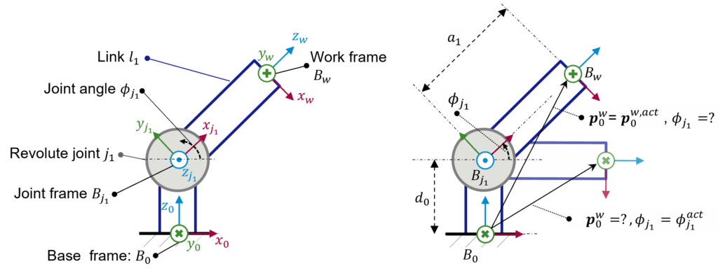
Before simulating the kinematics of a robot system, some essential mathematical concepts and the common terminology used in the context of kinematic modeling must be first understood. To this purpose, consider first a minimal system consisting of a revolute joint \(j_1\) and a link \(l_1\).
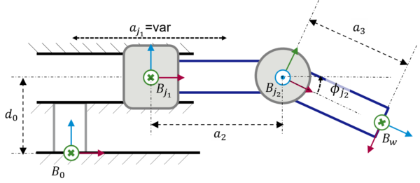
The link is rigidly coupled to the joint. This means that when the joint rotates over its z-axis (frame \(B_{j_1}\)) by an angle of \(\phi_{j_1}\) , link \(l_1\) rotates with it. Assume the system’s origin coordinate frame is located at the basis coordinate frame at \(B_0\). Moreover, the vector \(p_0^w := (x, y, z, a^x, \beta^y, \phi^z)^T\) describes the link’s pose (position and rotation) at the work frame \(B_w\). The 2D kinematic model of such system and its components are illustrated in left of Figure 1.
Figure 1: Simply kinematic model comprising one revolute joint and one link
Kinematic Model
Now, assuming that we will require to program or simulate some motions, we will inevitably be confronted with at least one of the following problems:
Inverse Kinematic Problem: Which is the angle \(\phi_{j1}\) corresponding to an actual pose \(p_0^{w,act}\)?
Forward Kinematic Problem: Which is the resulting link pose \(p_0^w\) of the actual joint angle \(\phi_{j1}^{act}\)?
These questions are depicted on the right of Figure 1 and represent the fundamental problems of kinematic modeling, denoted as the inverse and forward kinematic problems. To answer any of these questions, we first need to estimate all spatial relationships between all consecutive [1] frames of the system. That means from the base \(B_0\) to the joint \(B_{j1}\) and from the joint \(B_{j1}\) to the work frame \(B_w\). Let the relative spatial relationships[2] between two frames be modeled by the translational components \(x_{\Delta}, y_{\Delta}\), and \(z_{\Delta}\) and its rotational counterparts \(\alpha_{\Delta}^x\), \(\beta_{\Delta}^y\), and \(\phi_{\Delta}^z\). Table 1 shows the geometric relationships for all consecutive frames of the kinematic system of Figure 1.
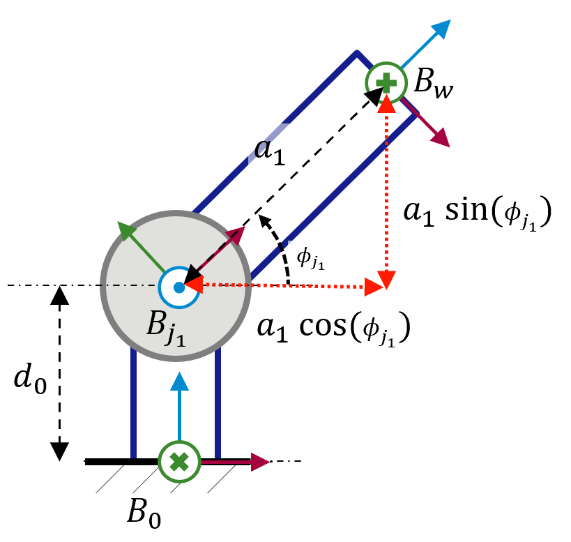
After having defined the geometrical relationships of our system, the kinematic model that will answer the previous questions can now be described. For example, the forward kinematic module that gives the resulting pose for a commanded joint angle could be modeled using the trigonometric relationships depicted in Figure 2.
Figure 2: Trigonometric relationships of reference system
\(x_0^w\) = \(a_1 \cos (\phi_{j1})\)
\(y_0^w\) = 0
\(z_0^w\) = \(d_0 + a_1 \sin (\phi_{j_1})\)
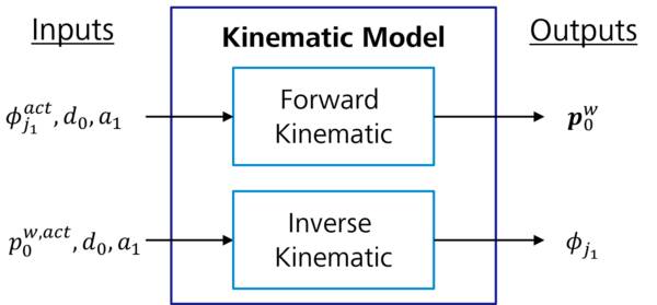
Although these geometric functions sufficiently model the kinematics of our reference system, it should be noted that describing the kinematic model in such a way is not so straightforward for more complex systems with multiple joints and links. For this reason, other mathematical approaches, e.g., homogenous matrices or quaternions, are generally used for computing multiple-coordinate transformations. The description of these techniques falls outside this blog’s scope. For the rest of the article, knowing which inputs and outputs we can expect from a kinematic model is sufficient. These models can be assumed as black-box components, as depicted in Figure 3.
Figure 3: Forward and inverse kinematic black-box models
Implementation
Now that the core concepts of kinematic modeling have been introduced, a seamless way of describing kinematic chains is introduced.
There exists a handful of specifications and formats that address the modeling of kinematic chains, e.g., Collada, AutomationML, OPC UA Robotics. However, in our experience, a standardized format has not been established within the industry. This represents a broader problem in the robotics domain, where programming languages are primarily vendor-specific, and there are no standards for programming or modeling robots. This is one of the reasons why the Robot Operating System (ROS) was founded in 2010. ROS is a FOSS robotics middleware that includes several libraries (e.g., kinematic modeling, perception, visualization, path planning) for hardware-agnostic programming of robotic systems. This has made ROS the state-of-the-art framework used within robotics research. Because of its popularity and characteristics (e.g., performance, hardware-agnostic, FOSS, modularity, SOA), manufacturers of robots, field devices (e.g., grippers and sensors), and software vendors have begun to offer programming interfaces for ROS.
As part of the development of ROS, the Unified Robot Description Format (URDF) was introduced for modeling kinematic chains. The URDF is an open standard XML schema for describing the geometric relationships between joints and links of a robot. In addition to modeling kinematic chains, the URDF provides the possibility to model the physical properties of joints (e.g., inertia, dynamics, and axis limits) or use CAD files for modeling the volumetric properties of links that can be used for collision testing. Furthermore, since the URDF follows an XML schema, kinematic models can be straightforwardly represented in a readable manner. For example, the following excerpt in Figure 4 describes the kinematic relationships between the joint j1 and the link l1 from Table 1.
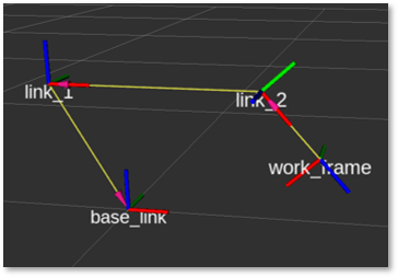
Having described the geometric relationships between all links and joints using a URDF file, the kinematic model can be visualized and used to calculate end-effector positions or required joint rotations. ROS integrates a handful of packages that use third-party libraries implementing all these functionalities. The use of these libraries is described in the ROS documentation.
<!--All links of our model.-->
<!--The root frame in ROS is called the base_link and represents the root frame (B_0) in our system. -->
<link name="base_link"/>
<!--The link 1 of our model. -->
<link name="link_1"/>
<!-- The work frame of our model is represented as a link.-->
<link name="work_frame"/>

<!--All joints of our model.-->
<!--The revolute joint 1, which couples the base link (parent link) with the link 1 (child link) is modeled here.
The joint is located at the origin of the child link.-->
<joint name="joint_1" type="revolute">
	<parent link="base_link"/>
	<child link="link_1"/>
<!-- Selection of rotation axis, in our case around the joint is around the z-axis in positive direction.-->
	<axis xyz="0 0 1"/>
<!-- The transformation between the parent and child link is given here.-->
<!-- The translational components (xyz) are given in meters. -->
<!-- The rotation is expressed by the Euler angles (rpy) in radians according to the following
 notation (r)oll (x-axis rot), (p)itch (y-axis rot.), and (y)aw (z-axis rot.). -->
	<origin xyz="0 0 0.4" rpy="1.57079632679 0.0 0.0"/>
<!-- The model of a movable joint must include further physical properties. -->
	<limit effort="100" lower="-0.175" upper="3.1416" velocity="0.5"/>
</joint>
Figure 4: URDF excerpt describing kinematic relationship between joint \(j_1\) and link \(l_1\)
Extended System
Having understood the basics of kinematic modeling and how to use URDFs to implement a kinematic model, nothing stands in the way of describing more complex multi-joint kinematic chains like the one shown in Figure 5.
Figure 5: Extended kinematic model considering a prismatic and a revolute joint.
The corresponding geometry relationships are given in Table 2. In addition, the complete URDF can be found attached.
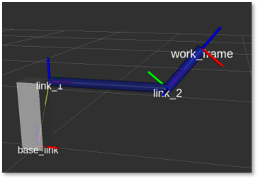
Figure 6: URDF visualization in ROS using two different joint configurations and following values: \(d_0\) = 300mm, \(a_2\) = 500mm, \(a_3\) = 200mm. The image on the right side also depicts the integration of surface models for modeling the volumetric properties of the links.
Summary and Outlook
Programming robots is a complex and resource-exhaustive task requiring expert knowledge, time, and in most cases, the use of the physical system. These barriers directly affect the software development and commissioning of such systems. A kinematic (mock) model of the robot enables the possibility of programming robots without requiring the physical system while reducing costs. However, modeling robot systems is considered a non-trivial task requiring in a first step that their kinematic model is described. For this reason, this blog introduced first the minimal mathematical fundamentals to understand kinematic modeling. Then, in a further step, we showed how kinematic models could be seamlessly implemented using the standard format URDF.
With the blogs’ insights, the reader should be able to describe kinematic models that can be used as mock-ups for prototyping or development purposes. Having overcome the first obstacle of kinematic modeling, the following steps might include:
offer kinematic models as microservices for development, testing, and commissioning purposes (further reading: Mocks in test environment)
develop more user-friendly programming frameworks based on kinematic simulations using cutting-edge technologies such as VR (virtual reality) or AR (augmented reality).
[1] For this reason, these models are commonly denoted as serial kinematic chains. There also exist parallel kinematic models for representing delta robots. The kinematic modeling of such systems lies outside the scope of this blog.
[2] In the robotic domain, the transformation between two coordinate frames is frequently described using homogenous transformations and a set of four parameters describing the translation and orientation displacement, known as the Denavit-Hartenberg parameters.


![Definition of digital model, shadow and twin based on flows of information[2]](https://blogs.zeiss.com/digital-innovation/en/wp-content/uploads/sites/3/2023/06/Folie1-1024x442.jpeg)