Kinematic Simulation for Beginners

Introduction

Mass individualized production, demographic change, labor shortage, and manufacturing reshoring are some global challenges that producing companies worldwide face. As a result, production sites in high-wage countries demand highly automated and flexible production systems to remain competitive. Industrial robots and custom machines have proven to be key assets and enablers in addressing some of these challenges. The flexible programming of these manufacturing systems allows tasks such as handling, transportation, and various production processes to be performed automatically with high precision, speed, and quality.

Although the benefits of such production systems have been widely demonstrated, it should be noted that there is a significant amount of integration and programming that must be considered before these systems can be run productively. In most cases, developing software for production systems requires using physical components under real conditions. However, the availability of such systems is limited in most cases for various reasons, e.g., the system is running, is being developed in parallel, or, in the worst case, does not exist. This problem causes software development to be delayed or postponed until the necessary physical components are available and integrated. In addition, programming an industrial robot is considered a non-trivial task that requires skilled operators with a good spatial understanding of the workspace and domain knowledge. Their main task is to program a sequence of motions that will ensure the completion of the production process while avoiding collisions and ensuring the process’s quality. For these reasons, industrial robot programming is still manually performed and considered challenging and resource-intensive.

At a more abstract level, these problems are common to software development in other domains. So the question arises: How do developers deal with these problems when there are no modules or interfaces? We create mocks! In a sense, mocks are nothing more than models that simulate a desired functionality. However, modeling a robot sounds a bit more complicated than mocking a database or an interface. This article aims to prove the opposite and presents a quick tutorial on how to create kinematic simulation models to make programming kinematic manufacturing systems more straightforward and efficient.

Takeaways for the reader:

• Basic understanding of kinematic simulation models.
• Ability to create a simple kinematic model of a manipulator (e.g., robot, rotary table, linear axes) based on Free and open-source software (FOSS) that can be used for prototyping, development, and testing purposes.

Kinematic Modelling

Reference System

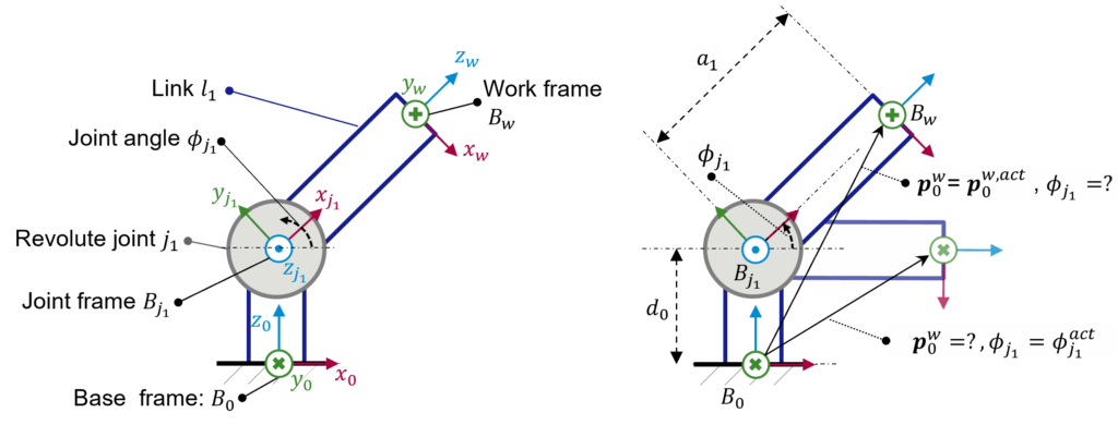
Before simulating the kinematics of a robot system, some essential mathematical concepts and the common terminology used in the context of kinematic modeling must be first understood. To this purpose, consider first a minimal system consisting of a revolute joint \(j_1\) and a link \(l_1\).

The link is rigidly coupled to the joint. This means that when the joint rotates over its z-axis (frame \(B_{j_1}\)) by an angle of \(\phi_{j_1}\) , link \(l_1\) rotates with it. Assume the system’s origin coordinate frame is located at the basis coordinate frame at \(B_0\). Moreover, the vector \(p_0^w := (x, y, z, a^x, \beta^y, \phi^z)^T\) describes the link’s pose (position and rotation) at the work frame \(B_w\). The 2D kinematic model of such system and its components are illustrated in left of Figure 1.

Kinematic Model

Now, assuming that we will require to program or simulate some motions, we will inevitably be confronted with at least one of the following problems:

• Inverse Kinematic Problem: Which is the angle \(\phi_{j1}\) corresponding to an actual pose \(p_0^{w,act}\)?
• Forward Kinematic Problem: Which is the resulting link pose \(p_0^w\) of the actual joint angle \(\phi_{j1}^{act}\)?

These questions are depicted on the right of Figure 1 and represent the fundamental problems of kinematic modeling, denoted as the inverse and forward kinematic problems. To answer any of these questions, we first need to estimate all spatial relationships between all consecutive ^[1] frames of the system. That means from the base \(B_0\) to the joint \(B_{j1}\) and from the joint \(B_{j1}\) to the work frame \(B_w\). Let the relative spatial relationships^[2] between two frames be modeled by the translational components \(x_{\Delta}, y_{\Delta}\), and \(z_{\Delta}\) and its rotational counterparts \(\alpha_{\Delta}^x\), \(\beta_{\Delta}^y\), and \(\phi_{\Delta}^z\). Table 1 shows the geometric relationships for all consecutive frames of the kinematic system of Figure 1.

Base Frame	Reference Frame	Translation	Rotation
Base \(B_0\)	Joint \(B_{j_1}\)	\(x_{\Delta}\) = 0, \(y_{\Delta}\) = 0, \(z_{\Delta}\) = \(d_0\)	\(\alpha_{\Delta}^x\) = 0, \(\beta_{\Delta}^y\) = 0, \(\phi_{\Delta}^z\) = \(\phi_{j_1}\)
Joint \(B_{j_1}\)	Work frame \(B_w\)	\(x_{\Delta}\) = \(a_1\), \(y_{\Delta}\) = 0, \(z_{\Delta}\) = \(d_0\)	\(\alpha_{\Delta}^x\) = -90°, \(\beta_{\Delta}^y\) = 0, \(\phi_{\Delta}^z\) = 0

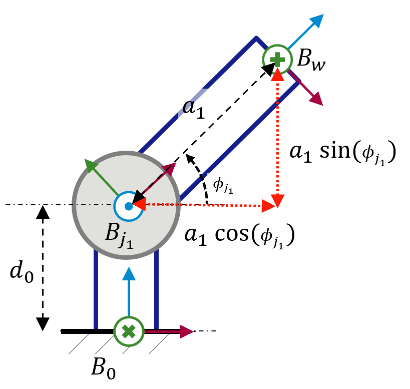
After having defined the geometrical relationships of our system, the kinematic model that will answer the previous questions can now be described. For example, the forward kinematic module that gives the resulting pose for a commanded joint angle could be modeled using the trigonometric relationships depicted in Figure 2.

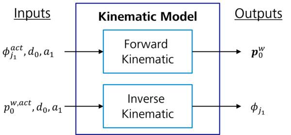
Although these geometric functions sufficiently model the kinematics of our reference system, it should be noted that describing the kinematic model in such a way is not so straightforward for more complex systems with multiple joints and links. For this reason, other mathematical approaches, e.g., homogenous matrices or quaternions, are generally used for computing multiple-coordinate transformations. The description of these techniques falls outside this blog’s scope. For the rest of the article, knowing which inputs and outputs we can expect from a kinematic model is sufficient. These models can be assumed as black-box components, as depicted in Figure 3.

Implementation

Now that the core concepts of kinematic modeling have been introduced, a seamless way of describing kinematic chains is introduced.

There exists a handful of specifications and formats that address the modeling of kinematic chains, e.g., Collada, AutomationML, OPC UA Robotics. However, in our experience, a standardized format has not been established within the industry. This represents a broader problem in the robotics domain, where programming languages are primarily vendor-specific, and there are no standards for programming or modeling robots. This is one of the reasons why the Robot Operating System (ROS) was founded in 2010. ROS is a FOSS robotics middleware that includes several libraries (e.g., kinematic modeling, perception, visualization, path planning) for hardware-agnostic programming of robotic systems. This has made ROS the state-of-the-art framework used within robotics research. Because of its popularity and characteristics (e.g., performance, hardware-agnostic, FOSS, modularity, SOA), manufacturers of robots, field devices (e.g., grippers and sensors), and software vendors have begun to offer programming interfaces for ROS.

As part of the development of ROS, the Unified Robot Description Format (URDF) was introduced for modeling kinematic chains. The URDF is an open standard XML schema for describing the geometric relationships between joints and links of a robot. In addition to modeling kinematic chains, the URDF provides the possibility to model the physical properties of joints (e.g., inertia, dynamics, and axis limits) or use CAD files for modeling the volumetric properties of links that can be used for collision testing. Furthermore, since the URDF follows an XML schema, kinematic models can be straightforwardly represented in a readable manner. For example, the following excerpt in Figure 4 describes the kinematic relationships between the joint j₁ and the link l₁ from Table 1.

Having described the geometric relationships between all links and joints using a URDF file, the kinematic model can be visualized and used to calculate end-effector positions or required joint rotations. ROS integrates a handful of packages that use third-party libraries implementing all these functionalities. The use of these libraries is described in the ROS documentation.

<!--All links of our model.-->
<!--The root frame in ROS is called the base_link and represents the root frame (B_0) in our system. -->
<link name="base_link"/>
<!--The link 1 of our model. -->
<link name="link_1"/>
<!-- The work frame of our model is represented as a link.-->
<link name="work_frame"/>

<!--All joints of our model.-->
<!--The revolute joint 1, which couples the base link (parent link) with the link 1 (child link) is modeled here.
The joint is located at the origin of the child link.-->
<joint name="joint_1" type="revolute">
	<parent link="base_link"/>
	<child link="link_1"/>
<!-- Selection of rotation axis, in our case around the joint is around the z-axis in positive direction.-->
	<axis xyz="0 0 1"/>
<!-- The transformation between the parent and child link is given here.-->
<!-- The translational components (xyz) are given in meters. -->
<!-- The rotation is expressed by the Euler angles (rpy) in radians according to the following
 notation (r)oll (x-axis rot), (p)itch (y-axis rot.), and (y)aw (z-axis rot.). -->
	<origin xyz="0 0 0.4" rpy="1.57079632679 0.0 0.0"/>
<!-- The model of a movable joint must include further physical properties. -->
	<limit effort="100" lower="-0.175" upper="3.1416" velocity="0.5"/>
</joint>

Figure 4: URDF excerpt describing kinematic relationship between joint \(j_1\) and link \(l_1\)

Extended System

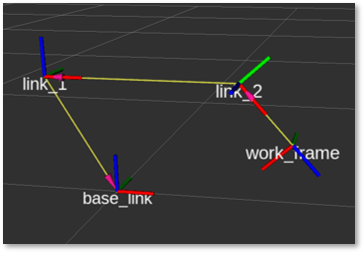
Having understood the basics of kinematic modeling and how to use URDFs to implement a kinematic model, nothing stands in the way of describing more complex multi-joint kinematic chains like the one shown in Figure 5.

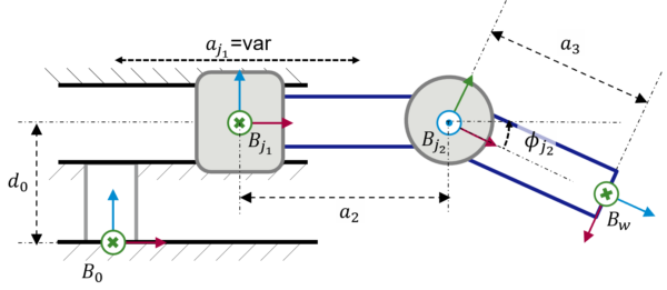
The corresponding geometry relationships are given in Table 2. In addition, the complete URDF can be found attached.

Base Frame	Reference Frame	Translation	Rotation
Base \(B_0\)	Joint \(B_{j_1}\)	\(\Delta x\) = \(a_{j_1}\), \(\Delta y\) = 0, \(\Delta z\) = \(d_0\)	\(\alpha_x\) = 0, \(\beta_y\) = 0, \(\phi_z = 0\)
Joint \(B_{j_1}\)	Joint \(B_{j_2}\)	\(\Delta\)x = \(a_2\), \(\Delta y\) = 0, \(\Delta z\) = 0	\(\alpha_x\) = 90°, \(\beta_y\) = 0, \(\phi_z\) = 0
Joint \(B_{j_2}\)	Work frame \(B_w\)	\(\Delta\)x = \(a_3\), \(\Delta y\) = 0, \(\Delta z\) = 0	\(\alpha_x\) = -90°, \(\beta_y\) = 0, \(\phi_z\) = 0

The URDF can then be straightforwardly used within ROS to visualize and position joints, as depicted in Figure 6.

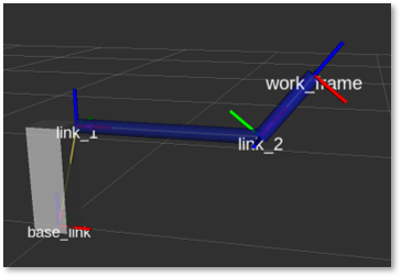
Figure 6: URDF visualization in ROS using two different joint configurations and following values:
\(d_0\) = 300mm, \(a_2\) = 500mm, \(a_3\) = 200mm. The image on the right side also depicts the integration of surface models for modeling the volumetric properties of the links.

Summary and Outlook

Programming robots is a complex and resource-exhaustive task requiring expert knowledge, time, and in most cases, the use of the physical system. These barriers directly affect the software development and commissioning of such systems. A kinematic (mock) model of the robot enables the possibility of programming robots without requiring the physical system while reducing costs. However, modeling robot systems is considered a non-trivial task requiring in a first step that their kinematic model is described. For this reason, this blog introduced first the minimal mathematical fundamentals to understand kinematic modeling. Then, in a further step, we showed how kinematic models could be seamlessly implemented using the standard format URDF.

With the blogs’ insights, the reader should be able to describe kinematic models that can be used as mock-ups for prototyping or development purposes. Having overcome the first obstacle of kinematic modeling, the following steps might include:

• integrate the kinematic model with a real robot system and build a digital twin (further reading: Smart Manufacturing, IOT with Azure Digital Twins)

• offer kinematic models as microservices for development, testing, and commissioning purposes (further reading: Mocks in test environment)

• develop more user-friendly programming frameworks based on kinematic simulations using cutting-edge technologies such as VR (virtual reality) or AR (augmented reality).

---

---

[1] For this reason, these models are commonly denoted as serial kinematic chains. There also exist parallel kinematic models for representing delta robots. The kinematic modeling of such systems lies outside the scope of this blog.

[2] In the robotic domain, the transformation between two coordinate frames is frequently described using homogenous transformations and a set of four parameters describing the translation and orientation displacement, known as the Denavit-Hartenberg parameters.

This post was written by: