Model Predictive Control Archives - Digital Innovation Blog

Data-driven Process Control – Part 3: Controlling System Behaviour

Manufacturing Solutions

This third and last part of the article series on data-driven process control provides an introduction to approaches for controlling systems. The focus is on the classic “model-predictive-control” scheme, which is combined with the results for system modeling from the second article to form a purely data-driven control strategy.

There are numerous theoretical and practical approaches to controlling systems. One of the simplest is the PID controller, which is used in applications such as motor and temperature control, charge control for solar systems or control units for power electronics.

However, we want to look at a more advanced control strategy for a wider range of applications, namely “Model Predictive Control (MPC)” (see [3] and [4]). As is evident from the name, this strategy presupposes the ability to predict the behaviour of the system. A requirement that can be fulfilled by modelling as described in the previous section, but also by the data-based approach presented.

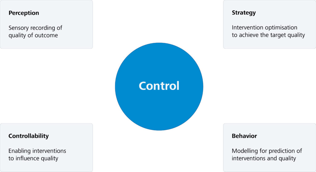
The purpose of the control strategy is to control the output target variables by modifying the intervention variables so that the former remain in a range determined by reference data.

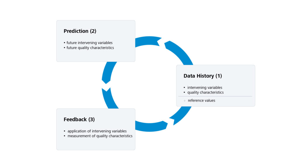
*Figure 1: The Model Predictive Control (MPC) Scheme*

The MPC strategy is an iterative process consisting of the following three phases (see also Figure 1).

The starting point is the historical data of the system to be controlled. This consists, firstly, of the values of the intervention parameters in previous control steps and, secondly, of the associated output data provided by the system. Since the reference data can also change over time, this makes up part of the historical data as well. This data base represents the status quo of the system under consideration. Any prediction of system behaviour must fit seamlessly into this history.
Starting with the existing system state, the model of the system is used to calculate an optimal prediction of future intervention variables and associated outputs. In this context, the decisive optimisation criterion is the requirement that the output of the system approximates the desired reference values as closely as possible in the prediction period under consideration (see “Mathematical background”). In addition, the technical boundary and limit conditions of the intervention parameters must be taken into account.
The third and final step is to apply the calculated intervention variables in the system itself. This takes the form of a practical test of the model used for prediction. Furthermore, the predicted intervention variables are not applied over the entire prediction horizon, but only for a few steps. This is done in the knowledge that any influences not taken into account by the model will falsify the feedback and thus limit the accuracy of the predictions. At the same time, the feedback ensures the robustness of the strategy, as the newly acquired data is incorporated into the data history and thus forms the updated basis for the next prediction.

The three phases described are run through cyclically. The frequency of this process is directly dependent on the requirements of the particular application. Especially in the case of controlling real-time systems such as vehicles and aircraft, frequencies in the 10 Hz range or beyond are necessary.

Mathematical background

The central element of the “Model Predictive Control” scheme is the prediction of future input parameters $u_f$ and output variables $y_f$ , which minimise the distance to a reference trajectory $w_r = (u_r, y_r)$ in the prediction time horizon $T_f$ . In addition, historical data is given in the form of an initial trajectory $w_\text{ini} = (u_\text{ini}, y_\text{ini})$ of length $T_\text{ini}$ , which is to be extended by the sought trajectory $w_f = (u_f, y_f)$ .

Figure 2: Prediction in the Model Predictive Control scheme

Since the algebraic representation $H_L$ of the time-restricted behaviour $B_L$ allows to determine a vector $g$ for each $w \in B_L$ , to which $H_L \, g = w$ applies, we can formulate the following constrained optimisation problem for $w_f$

$\begin{aligned} &\underset{g}{\text{minimize}} \quad \| H_{T_f} \ g - w_r \|^2_2 & \\[1.0em] &\text{subject to} \quad H_{T_\text{ini}} \ g = w_\text{ini}, & \end{aligned}$

using the decomposition

$H_L \, g = w \quad \Longleftrightarrow \quad \begin{bmatrix} H_{T_\text{ini}} \\[0.5em] H_{T_f} \end{bmatrix} \, g= \begin{bmatrix} w_\text{ini} \\[0.5em] w_f \end{bmatrix}$

The constraint ensures compliance with the initial condition and the use of $H_{T_f} \ g$ in the minimisation functional ensures that the determined future trajectory $w_f = H_{T_f} \ g$ is permissible for the system $S$ . In addition, constraints on $w_f$ can be formulated, which was not done in this case for reasons of clarity. Further details are provided in [2] and [7].

The robustness of this scheme to disturbances in the form of non-modelled system behaviour can be proven mathematically. In particular, it is ensured that the optimisation problem posed in step 2 remains solvable in each subsequent cycle, provided it was solvable in the first cycle. This guarantees that the procedure can be carried out without any restrictions (see [5] and [6]).

Summary

Control of physical systems requires a priori knowledge, which is introduced into the control task by system models. Conventional approaches to modelling encounter fundamental limits as the complexity of the system increases. However, they provide essential theoretical insights into the structure of the system during their creation and require only little prior experimental knowledge.

The data-based approach presented here, on the other hand, generates a system representation from a single series of observations obtained by subjecting the system to a specific type of stimulation. The completeness of the system representation generated can be checked against the data already obtained, which is a remarkable feature for a learning procedure. This approach means that the method is not subject to any fundamental restrictions with regard to system complexity, but instead requires special empirical data for system description purposes.

Although the new approach does not deliver a model in the true sense, the system representation it generates allows specific predictions to be made about the system’s behaviour. Not only is convergence towards a desired target state achieved, but technical and physical restrictions are also implemented on the input and output sides. This represents a significant advantage over other learning methods and facilitates safety-critical applications in conjunction with established control strategies such as “Model Predictive Control”.

Outlook

The presentation of the new data-based approach has left out the treatment of two major problems.

The first aspect concerns the application to non-linear systems. According to theoretical requirements, the data-based approach is limited to linear time-invariant systems. On the one hand, there have been recent attempts, as in [1] or [4], to overcome this limitation. On the other hand, the reasons why the data-based approach has proven successful in controlling non-linear systems are not yet understood and are therefore the subject of current research, see [2].

The second aspect relates to the use of noisy observation data in the reconstruction of system behaviour. Here, too, significant progress has already been made towards stabilising data-based approaches, see [2]. Nevertheless, other approaches to system identification are still proving to be far less sensitive to noise influences.

Overall, the picture emerges that current data-based methods are robust against bias data errors, i.e. data from non-linear systems, and more vulnerable to variance data errors, i.e. data noise.

Literature

[1] Ezzat Elokda, Jeremy Coulson, Paul N. Beuchat, John Lygeros, and Florian Dörfler, “Data-enabled predictive control for quadcopters”, International Journal of Robust and Nonlinear Control, 2021

[2] Florian Dörfler, Jeremy Coulson, and Ivan Markovsky, “Bridging direct and indirect data-driven control formulations via regularizations and relaxations”, IEEE Transactions on Automatic Control, 2022

[3] James B. Rawlings, David Q. Mayne, and Moritz M. Diehl, “Model predictive control – theory, computation, and design”, Nob Hill Publishing, 2022

[4] Julian Berberich, Johannes Köhler, Matthias A. Müller, and Frank Allgöwer, “Data-driven model predictive control – closed-loop guarantees and experimental results”, at-Automatisierungstechnik, 2021

[5] Joscha Bongard, Julian Berberich, Johannes Kohler, and Frank Allgower, “Robust stability analysis of a simple data-driven model predictive control approach”, IEEE Transactions on Automatic Control, 2022

[6] Julian Berberich, Johannes Köhler, Matthias A. Müller, and Frank Allgöwer, “Stability in data-driven MPC – an inherent robustness perspective”, IEEE Conference on Decision and Control, 2022

[7] Ivan Markovsky and Florian Dörfler, “Behavioral systems theory in data-driven analysis, signal processing, andcontrol”, Annual Reviews in Control, 2021

Data-driven Process Control – Part 2: Modelling System Behaviour

Manufacturing Solutions

After the first article in this series dealt with the general basic building blocks of control systems, the second article is dedicated to modeling the behavior of systems. The focus here is on differentiating between different types of modeling. The main part of the article introduces a special data-driven approach that has recently attracted growing scientific interest.

Knowledge of the system behaviour, i.e. knowledge of the quantitative change in output when the system’s inputs change, is a basic prerequisite for system control. This knowledge is represented by behavioural models, the development of which we will examine in more detail in this section.

A physical example system

As a simple physical example, let’s look at what is known as an ideal planar pendulum. The pendulum mass is assumed to be point-like and suspended on a massless cord; all frictional forces are disregarded. The only force acting on the mass is the gravitational force of the Earth (see Figure 3).

Figure 3: The ideal pendulum

We will use this example to describe three basic types of modelling.

Whitebox Modelling

In this type of modelling, the system behaviour is represented by differential equations whose parameters are completely known. The approach is highly application-specific and requires a high degree of detailed knowledge of the system under consideration. The complexity of real-life systems obviously places limits on the application of this approach. In addition, the strategy is difficult to automate and the models ob

We will use this example to describe three basic types of modelling.tained are difficult to adapt to changing requirements.

Example – white box modelling of the pendulum system

The starting point is Newton’s second law $F = m \, a$ and Newton’s law of gravitation, specifically for bodies near the Earth’s surface $F = m \, g \, [\, 0, -1 \,]^T$ . In terms of the motion of the pendulum, only the force $F_T$ acting tangentially on the pendulum mass is to be considered, since the radial component is compensated by the cord. For the same reason, only the tangential acceleration $a_T$ is relevant. Using the time-dependent deflection angle $\theta(t)$ and the angular acceleration $\ddot{\theta}(t)$ (see Figure 3), the variables $F_T$ and $a_T$ are given as

$F_T = -m \ g \sin \theta(t) \quad \text{and} \quad a_T(t) = l \, \ddot{\theta}(t)$

with the length $l$ of the pendulum cord and $g \approx 9.81 \frac{m}{s^2}$ as the gravitational acceleration on Earth. Therefore, $m \ a_T = F_T$ results in the following differential equation for the deflection angle $\theta$

$\ddot{\theta} (t) = - \frac{g}{l} \ \sin \theta(t)$

If we additionally assume that the angle $\theta$ is small, we obtain as a further simplification

$\ddot{\theta} (t) = - \frac{g}{l} \ \theta(t)$

This differential equation can be used to predict the behaviour of the pendulum for any initial angle $\theta_0 \ll 1$ and any initial velocity $\dot{\theta}_0$ .

Grey- and Blackbox Modelling

This modelling approach also results in differential or difference equations, which, however, only specify the basic structure of the system and therefore contain free parameters. If the system model incorporates prior knowledge, for example in the form of physical principles, then it is a grey box model. Otherwise it is referred to as a black box model.

The free parameters of the model are determined from observed data of the system during an adaptation step, whereby this step of the modelling can be automated to a large extent. The choice of model structure, however, is critical for the quality of the model, requires a high degree of experience due to its complexity and can therefore only be automated to a limited degree. Moreover, in contrast to the white box approach, grey and black box modelling can be applied to systems of any complexity.

Data-Based Modelling

This new approach has been attracting an increasing amount of attention for some years now. The starting point is the notion of identifying a system solely on the basis of its externally verifiable behaviour. A detailed description of the systems-theoretical background for this approach can be found in [1]. With the increasing availability of process data from technical systems, the view of this data-driven approach has changed. It was recognized that the description of system behavior based purely on observations opened the door to new models and algorithms (see [2] and [3]). This transition is comparable to developments in the application of neural networks in recent years.

Since it is an unsupervised learning procedure for non-parametric system representations, no model of the system is constructed, unlike in white, grey and black box modelling. As such, the applicability of this approach is not subject to complexity-related limitations, nor does the need for a structural decision prevent it from being automated. That said, the approach is initially limited to so-called linear and time-invariant systems (see “Mathematical background”).

Example – Data-based modelling of the pendulum system

To arrive at a data-based representation for the pendulum system, we only need to conduct two experiments. Using the notation $x(t) = [\, \theta(t), \dot{\theta}(t) \, ]^T$ with the deflection angle $\theta(t)$ and the angular velocity $\dot{\theta}(t)$ , the initial conditions for the two experiments can be taken as

$x_1(0) = \begin{bmatrix} 1 \\ 0 \\ \end{bmatrix} \quad \text{and} \quad x_2(0) = \begin{bmatrix} 0 \\ 1 \\ \end{bmatrix}$

The first experiment records the motion $x_1(t)$ of the pendulum at the starting angle $1^{\circ}$ and vanishing starting velocity at discrete points in time $\{ t_i \}_{i=1}^n$ . The second experiment uses the inverse setting for recording $x_2(t)$ .

The recordings of both experiments can then be used to calculate any other pendulum motion $x(t)$ at the initial conditions $x(0) = [\, \theta_0, \dot{\theta}_0 \,]^T$ by means of the relationship

$x(t) = \theta_0 \ x_1(t) + \dot{\theta}_0 \ x_2(t)$

at the points in time $\{ t_i \}_{i=1}^n$ , whereby the linear independence of the vectors of the two initial conditions is essential. Further we obtain the compact representation

$B \, x(0) = x \quad \text{with} \quad B = \begin{bmatrix} x_1(t_1) & x_2(t_1) \\ \vdots & \vdots \\ x_1(t_n) & x_2(t_n) \end{bmatrix} \quad \text{and} \quad x = \begin{bmatrix} x(t_1) \\ \vdots \\ x(t_n) \end{bmatrix}$

We call the matrix $B$ an algebraic representation of the pendulum behavior.

The objective of reconstructing the entire system behaviour from observed data alone raises three main questions:

What data is suitable for behavioural representation?
How can this suitability be verified?
What is the scope of the collected data?

The mathematical theory provides clear answers to these questions (see “Mathematical background”). At this point, we will limit ourselves to stating that the collected data must have a level of independence that is precisely mathematically defined (see Example – Data-based modelling of the pendulum system). Such data can only be obtained by systematically stimulating the system, as physical systems naturally tend to transition into a state of equilibrium after some time in the absence of disturbances.

The necessary course of action is therefore to stimulate the system by means of random inputs during the observation period, thereby inducing the most diverse output behaviour possible (see Figure 4). It should be noted that this system stimulation must be carried out in compliance with the technical boundary and limit conditions of the system in order to avoid destabilisation with potentially serious consequences.

Figure 4: Random inputs for exploring system behaviour

At regular intervals, a dimensional criterion is used to check whether the collected data already encompasses all of the possible system responses. This check requires the desired or presumed system complexity to be specified (see “Mathematical background”), which includes the possibility of limiting it to a desired level. If the amount of data collected up to that point does not yet have the required complexity, random input data is generated again and the experiment is repeated.

As a result of this procedure, a system representation is generated from the observed data collected. In addition to being able to dynamically adapt the complexity of the system representation, the decisive advantage of this procedure is that the process described can be fully automated and therefore repeated autonomously if required.

The representation of the system behaviour obtained can now be used to make predictions about the system behaviour in the same way as the procedure outlined in the example “Data-based modelling of the pendulum system”. An example of how the method is used for quadcopter position control can be found in [4].

Mathematical background

The process under consideration is described as a linear and time-invariant dynamic system $S$ , which has $m$ input parameters, $p$ output variables and $n$ internal states and satisfies a difference equation of the form

$\begin{aligned} x(k+1) &= A \, x(k) + B \, u(k) \\[0.5em] y(k) &= C \, x(k) + D \, u(k) \end{aligned}$

with $x(k) \in \mathbb{R}^n$ , $u(k) \in \mathbb{R}^m$ , and $y(k) \in \mathbb{R}^p$ .

The behaviour $B$ of the system is defined as the set of all trajectories $w = (u, y)$ , the time-restricted version $B_L$ , consisting of trajectories of length $L$ , is identified with a finite-dimensional vector space of the dimension

$\dim B_L = m L + n.$

Through observation and excitation of the system $S$ , a matrix $H_L$ is formed as part of the identification process, the columns of which correspond to trajectories of length $L$ . Knowing the dimension of $B_L$ allows to check whether the columns of $H_L$ already collected span a sufficiently high-dimensional subspace before deciding to stop data acquisition.

The number $n$ of internal states of the system $S$ is regarded as a complexity measure for the system to be identified, and can be used to limit the complexity of the empirically determined system representation $H_L$ of $B_L$ in order to adapt the accuracy of the approximation to the requirements.

Having familiarised ourselves with the development of system models, especially for the purely data-driven case, we will now turn to the topic of control in the following section. The focus will be on a strategy that is particularly suited to control highly complex systems, i.e. systems with a large number of intervention and target variables.

Sources

[1] Jan C. Willems, “Paradigms and puzzles in the theory of dynamical systems”, IEEE Transactions on Automatic Control, 1991

[2] Ivan Markovsky, Linbin Huang, and Florian Dörfler, “Data driven control based on the behavioral approach – from theory to applications in power systems”, IEEE Control Systems, 2022

[3] Ivan Markovsky and Florian Dörfler, “Behavioral systems theory in data-driven analysis, signal processing, and control”, Annual Reviews in Control, 2021

[4] Ezzat Elokda, Jeremy Coulson, Paul N. Beuchat, John Lygeros, and Florian Dörfler, “Data-enabled predictive control for quadcopters”, International Journal of Robust and Nonlinear Control, 2021

Data-driven process control – Part 1

Manufacturing Solutions

Automatic control of complex physical systems is an ever-growing theoretical and technical challenge for scientists and engineers. To begin with, it is irrelevant whether these systems are biological or chemical reactors, wind turbines, power grids, aircraft or even manufacturing systems. In all of these use cases, similar theoretical and practical issues come to the fore. We will look at some of the key ones in more detail in this article. Before we can start, however, we need more prior knowledge.

In the following, we will discuss the relevant aspects mostly in descriptive or graphical form. A highly condensed, schematic mathematical description will be provided in suitably differentiated sections, which should at least give a brief insight into the relevant theoretical background.

A production-related example

Idealised workpiece machining on a turning machine, as shown in Figure 1, will serve as an example of a simple system that needs to be controlled.

Figure 1: Workpiece machining on a turning machine

The rotationally symmetrical workpiece (1) to be machined performs a rotational movement, which makes it possible to reduce the workpiece diameter D by removing material with the tool (2). The tool is fed in accordance with the CNC program so that material is removed until the desired diameter D is achieved.

The tool is mounted on a fixture (3) which is positioned at a distance C from the centre of rotation. This distance C can be adjusted to compensate for tool wear.
As we will see below, this simple example is enough to identify the essential components of an automatic control system in the next section.

Basic components of control systems

Automatic control of a system requires four central components to be available to solve this task. The first requirement is to define and automatically record target variables that are to be subjected to control. Secondly, the system must possess intervention variables that allow these target variables to be manipulated. Thirdly, it is necessary to understand the quantitative relationship between the target variables and the intervention variables of the system. The fourth requirement is a strategy for adjusting the intervention variables that is capable of steering the target variables into a range determined a priori and keeping them there.

Figure 2 gives an overview of the basic components required for automatic control, which we will look at in more detail below.

Perception

For some time now, an increasing number of measurement systems have been integrated directly into production lines and manufacturing machines. This makes it possible to capture the quality and process data generated in the manufacturing process at the frequency and density required for effective control. Moreover, the latest research projects are attempting to supplement or replace these measurement systems with so-called virtual measurement technology. These techniques rely on the extraction of quality data from process data using a digital twin of the manufacturing process.

In our example system, the objective is to automatically measure the diameter of the workpiece after production, for example using a laser scanner. In a more complex stage of expansion, the workpiece surface can be digitised in 3D.

Controllability

In most cases, it is possible to control manufacturing systems at a fundamental level for reasons of practicality. This means that the operator is able to intervene in manufacturing systems and machines in order to control quality-relevant target variables. That said, the ability to automate these interventions is still lacking in many cases, as they often interfere with safety-critical systems. It could also be the case that this feature was simply not envisaged.

In our example system, the distance C is the necessary intervention variable. By changing C, the feed distance stored in the CNC program can be adapted to the tool wear. As a rule, however, this change still needs to be made manually by the machine operator.

Behaviour

To control the system, it is essential to know how the system’s target variables change when the system’s intervention variables are manipulated. These relationships are summarised in models of system behaviour and can be extremely complex, which is why this aspect of control is a key challenge.

In our example system, the relationship is between the distance C and the final diameter D. This relationship is clearly a linear one, as the tool is at the same height as the axis of rotation. If this were not the case, it would be a non-linear relationship.

Strategy

The control strategy is responsible for controlling the target variables by adjusting the intervention variables. The relationship between these variables is established by the model used. Reference values and tolerance ranges are available for the target variables, and these must be adhered to for the purposes of quality assurance.

As the system model is inherently incomplete, it is necessary to adapt and correct it as part of the control strategy by means of feedback from the system. Furthermore, the chosen strategy must be able to withstand system disturbances caused by changes in non-modelled external and internal variables in order to ensure that the control objective is achieved despite these influences.

The control strategy for our example system is obvious. As soon as the automatic measurement of the diameter D reveals a deviation from the desired diameter, the distance C is adjusted by the value of this deviation using the opposite sign. However, this approach neglects aspects such as systematic and random measurement errors, which limits the robustness of the method.

As is evident from the above explanations, the aspects of behaviour and strategy pose a particular challenge, both in practical and theoretical terms. For this reason, we will focus on both of these topics in the following two articles. In the next article we will address, among other things, the possibility of automatic modelling of highly complex technical systems, and in the final article we will deal with the development of corresponding robust control strategies.